The method we use in Radiance for reducing the number of shadow rays is described in [26]. A prioritized list of potential source contributions is created at each evaluation of Equation (1). The largest potential contributors (contribution being a function of source output, proximity and BRDF) are tested for shadows first, and we stop testing when the remainder of the source list is below some fraction of the unoccluded contributions. The remaining source contributions are then added based on statistical estimates of how likely each of them is to be visible.
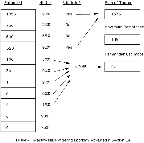
Figure 4 shows a simple example of how this works. The left column represents our sorted list of potential light source contributions for a specific sample point. We proceed down our list, checking the visibility of each source by tracing shadow rays, and summing together the unobstructed contributions. After each test, we check to see if the remainder of our potential contributions has fallen below some specified fraction of our accumulated total. If we set our accuracy goal to 10%, we can stop testing after four light sources because the remainder of the list is less than 10% of our known direct value. We could either add all of the remainder in or throw it away and our value would still be within 10% of the correct answer. But we can do better than that; we can make an educated guess at the visibility of the remaining sources using statistics. Taking the history of obstructed versus unobstructed shadow rays from previous tests of each light source, we multiply this probability of hitting an untested source by the ratio of successful shadow tests at this point over all successful shadow tests (2/(.9+.55+.65+.95) == 0.65 in this example), and arrive at a reasonable estimate of the remainder. (If any computed multiplier is greater than 1, 1 is used instead.) Our total estimate of the direct contribution at this point is then the sum of the tested light sources and our statistical estimate of the remainder, or 1616 in this example.
We have found this method to be very successful in reducing the number of shadow test rays required, and it is possible to place absolute bounds on the error of the approximation. Most importantly, this type of adaptive shadow testing emphasizes contrast as the primary decision criterion. Contrast is defined as the difference between the luminance at a point and the background luminance divided by the background luminance. If a shadow boundary is below the visible contrast threshold, then an error in its calculation is undetectable by the viewer. Thus, this method produces no visible artifacts in its tradeoff of speed for accuracy. Accuracy is still lost in a controlled way, but the resulting image is subjectively flawless, due to the eye's relative insensitivity to absolute light levels.
Figure 5 shows a theater lighting simulation generated by Radiance in 1989. This image contains slightly over a hundred light sources, and originally took about 4 days to render on a Sun-4/260. (The equivalent of about 5 Vax-11/780's.) Using our adaptive shadow testing algorithm reduced the rendering time to 2 days for the same image. The time savings for scenes with more light sources can be better than 70%, especially if the light sources have narrow output distributions, such as the spotlights popular in overlighted retail applications.
A different problem associated with ray-per-source shadow testing is inadequate sampling of large or nearby sources, which threatens simulation accuracy. For example, a single ray cannot adequately sample a fluorescent desk lamp for a point directly beneath it. The simplest approach for sources that are large relative to their distance is to send multiple sample rays. Unfortunately, breaking a source into pieces and sending many rays to it is inefficient for distant points in the room. Again, an adaptive sampling technique is the most practical solution.
In our adaptive technique, we send multiple rays to a light source if its extent is large relative to its distance. We recursively divide such sources into smaller pieces until each piece satisfies some size/distance criterion. Figure 6a shows a long, skinny light source that has been broken into halves repeatedly until each source is small enough to keep penumbra and solid angle errors in check. Figure 6b shows a similar subdivision of a large rectangular source. A point far away from either source will not result in subdivision, sending only a single ray to some (randomly) chosen location on the source to determine visibility.